授業で扱う資料 (Education)

Quarto資料

授業中に扱う題材をまとめています。¹

予測・分類・推定・検定・回帰などの基本的な概念を理解するための題材を扱います。

1. 年収に関する解析？

予測と推定の違いを理解する

まずはデータベースを作る。

何らかのsamplingを行い、一人づつ年収や資格の有無、年齢、性別、学歴などを記録して、c(200,1,25,1,0)のような形でデータを記入していく。

ここでは便宜上、年収と年齢を数値、資格と性別と学歴を二値という形を、データ定義書で決めているとする。

name <- c("nensyu","shikaku","age","gender","gakureki")
X1 <- rbind(
   c(200,1,25,1,0)
  ,c(300,1,30,1,1)
  ,c(200,0,27,0,0)
  ,c(240,0,26,0,1)
  ,c(180,0,23,1,0)
  ,c(650,1,27,1,1)
  ,c(550,1,30,1,1)
  ,c(600,1,24,1,1)
  ,c(580,1,26,0,1)
)
colnames(X1) <- name
rownames(X1) <- 1:nrow(X1)
X1 <- data.frame(X1)
X1$gender   <- as.factor(X1$gender)
X1$shikaku  <- as.factor(X1$shikaku)
X1$gakureki <- as.factor(X1$gakureki)
head(X1)

  nensyu shikaku age gender gakureki
1    200       1  25      1        0
2    300       1  30      1        1
3    200       0  27      0        0
4    240       0  26      0        1
5    180       0  23      1        0
6    650       1  27      1        1

目視で、データベース完成してそうな事を確認した。

Table.1

次は、集計する。資格の有無で各テーブルに差はないか？

library(tableone)
CreateTableOne(vars = c("age","gender","gakureki","nensyu"), 
               strata = c("shikaku"), 
               data = X1
               )

                    Stratified by shikaku
                     0              1               p      test
  n                       3              6                     
  age (mean (SD))     25.33 (2.08)   27.00 (2.53)    0.361     
  gender = 1 (%)          1 (33.3)       5 (83.3)    0.453     
  gakureki = 1 (%)        1 (33.3)       5 (83.3)    0.453     
  nensyu (mean (SD)) 206.67 (30.55) 480.00 (183.85)  0.043

これがいわゆる素データの比較（単変量解析）で、資格の有無で年収や年齢などに差があるかをみている。

解析

今、何のために解析ソフトを回しているのか、を再度考えてみましょう。

summary(lm(nensyu~shikaku,data=X1))


Call:
lm(formula = nensyu ~ shikaku, data = X1)

Residuals:
    Min      1Q  Median      3Q     Max 
-280.00  -26.67   33.33  100.00  170.00 

Coefficients:
            Estimate Std. Error t value Pr(>|t|)  
(Intercept)    206.7       90.2   2.291   0.0557 .
shikaku1       273.3      110.5   2.474   0.0426 *
---
Signif. codes:  0 '***' 0.001 '**' 0.01 '*' 0.05 '.' 0.1 ' ' 1

Residual standard error: 156.2 on 7 degrees of freedom
Multiple R-squared:  0.4665,    Adjusted R-squared:  0.3903 
F-statistic: 6.121 on 1 and 7 DF,  p-value: 0.04257

summary(lm(nensyu~shikaku+gender+age+gakureki,data=X1))


Call:
lm(formula = nensyu ~ shikaku + gender + age + gakureki, data = X1)

Residuals:
      1       2       3       4       5       6       7       8       9 
-118.98 -155.12   98.11 -118.98   20.87  134.41   94.88   23.94   20.87 

Coefficients:
            Estimate Std. Error t value Pr(>|t|)
(Intercept)   646.09     635.88   1.016    0.367
shikaku1      200.16     152.51   1.312    0.260
gender1       -23.39     130.54  -0.179    0.867
age           -20.16      25.15  -0.801    0.468
gakureki1     236.93     136.85   1.731    0.158

Residual standard error: 150.4 on 4 degrees of freedom
Multiple R-squared:  0.7174,    Adjusted R-squared:  0.4348 
F-statistic: 2.539 on 4 and 4 DF,  p-value: 0.1944

推定か予測かによって、結果で着目する所が違うので、どこをみて解析結果をどのように解釈しているかを覚えておきましょう。

Tip

どのようにデータを集めてきたのか、によって話が全然違ってくる、という事も理解できればなおよしです。

2. コイントスを何度行えばイカサマに気づく？

検定とは何かを理解する

あなたは何回コインが表が出たら、イカサマコインだと判定しますか？

まずは仮説が必要

「普通のコインって表裏平等に出るんじゃないか？」を検証する

上から1回目とし、表をo、裏をxと表現するとし、5回コイントスを行う全パターンを考える。

5回の時

# Tree drawing function
draw_tree <- function(depth, x, y, dx, heads = 0) {
  if (depth == 0) {
    # Bottom: print number of heads (non-overlapping)
    text(x, y, heads, cex = 0.9, col = "blue", font = 2)
  } else {
    x_left <- x - dx
    x_right <- x + dx
    y_next <- y - 1
    
    segments(x, y, x_left, y_next)
    segments(x, y, x_right, y_next)
    
    text((x + x_left)/2, (y + y_next)/2, "o", pos = 3, cex = 0.8)
    text((x + x_right)/2, (y + y_next)/2, "x", pos = 3, cex = 0.8)
    
    draw_tree(depth - 1, x_left, y_next, dx / 2, heads + 1)
    draw_tree(depth - 1, x_right, y_next, dx / 2, heads)
  }
}

# Set plotting area for the tree
par(mfrow = c(2, 1), mar = c(4, 4, 3, 2))

# Tree structure
plot(0, 0, type = "n", xlim = c(-16, 16), ylim = c(-6.5, 1.5),
     xlab = "", ylab = "", axes = FALSE, main = "Coin Toss Tree (5 flips)")

# Draw tree
draw_tree(depth = 5, x = 0, y = 1, dx = 8)

# Generate simulation data
set.seed(42)
n_trials <- 1000
sim_result <- rbinom(n_trials, size = 5, prob = 0.5)

# Plot probability density function
density_obj <- density(sim_result, from = -0.5, to = 5.5)

plot(density_obj, main = "Empirical Density of 'o' in 1000 Trials",
     xlab = "Number of 'o' ", ylab = "Density", col = "darkgreen", lwd = 2)
rug(sim_result, col = "gray")

このふにゃふにゃは？

全パターンが、\(2^5=32\)なので、\(1 \div32=0.03125\)となるので、全部表になった場合は0.05以下にはなっている。

# Simulate coin toss outcomes
set.seed(42)
n_trials <- 1000
sim_result <- rbinom(n_trials, size = 5, prob = 0.5)

# Smooth density estimation (adjust controls smoothness)
density_obj <- density(sim_result, from = -0.5, to = 5.5, adjust = 3)#滑らかに

# Plot density
plot(density_obj, main = "Smoothed Density of 'Heads' in 1000 Trials",
     xlab = "Number of Heads", ylab = "Density", col = "darkgreen", lwd = 2)
rug(sim_result, col = "gray")

８回くらいに増やすと、、、

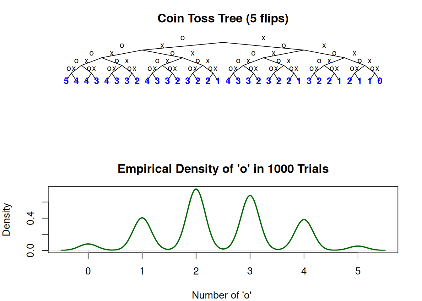
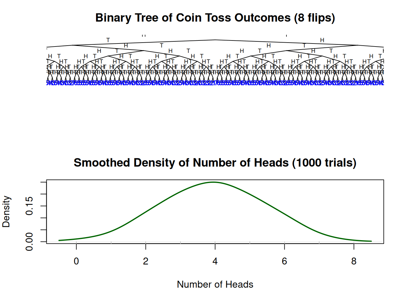
# Function to draw coin toss tree
draw_coin_tree <- function(depth, x_pos, y_pos, dx, num_heads = 0) {
  if (depth == 0) {
    text(x_pos, y_pos, num_heads, cex = 0.7, col = "blue", font = 2)
  } else {
    x_left <- x_pos - dx
    x_right <- x_pos + dx
    y_next <- y_pos - 1

    segments(x_pos, y_pos, x_left, y_next)
    segments(x_pos, y_pos, x_right, y_next)

    text((x_pos + x_left)/2, (y_pos + y_next)/2, "H", pos = 3, cex = 0.6)
    text((x_pos + x_right)/2, (y_pos + y_next)/2, "T", pos = 3, cex = 0.6)

    draw_coin_tree(depth - 1, x_left, y_next, dx / 2, num_heads + 1)
    draw_coin_tree(depth - 1, x_right, y_next, dx / 2, num_heads)
  }
}

# Parameters
num_flips <- 8
num_simulations <- 1000
set.seed(42)

# Simulate coin toss outcomes (number of heads per trial)
head_counts <- rbinom(num_simulations, size = num_flips, prob = 0.5)

# Prepare 2-panel layout
par(mfrow = c(2, 1), mar = c(4, 4, 3, 2))

# Plot the coin toss tree
plot(0, 0, type = "n", xlim = c(-140, 140), ylim = c(-9.5, 1.5),
     xlab = "", ylab = "", axes = FALSE,
     main = "Binary Tree of Coin Toss Outcomes (8 flips)")

draw_coin_tree(depth = num_flips, x_pos = 0, y_pos = 1, dx = 128)

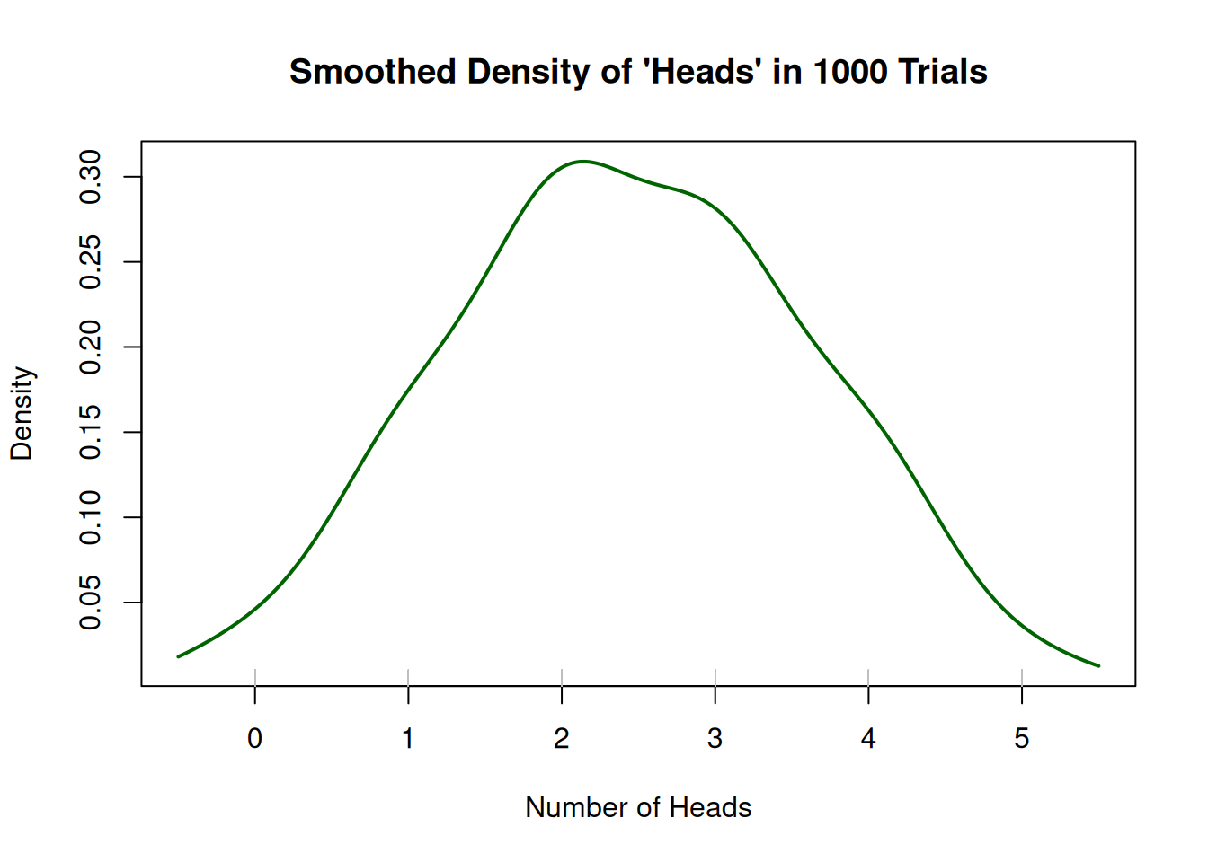
# Estimate and plot smoothed density of head counts
head_density <- density(head_counts, from = -0.5, to = 8.5, adjust = 2)

plot(head_density, main = "Smoothed Density of Number of Heads (1000 trials)",
     xlab = "Number of Heads", ylab = "Density", col = "darkgreen", lwd = 2)
rug(head_counts, col = "gray")

1000だとどうなるか？

# Parameters
num_flips <- 1000
num_simulations <- 10000  # 増やすことで密度が安定

set.seed(42)
head_counts <- rbinom(num_simulations, size = num_flips, prob = 0.5)

# Estimate smoothed density of head counts
head_density <- density(head_counts, from = 300, to = 700, adjust = 2)

# Plot density
par(mar = c(5, 4, 3, 2))  # Default margins
plot(head_density,
     main = "Smoothed Density of 'Heads' in 10000 Trials (100 Coin Flips)",
     xlab = "Number of Heads", ylab = "Density",
     col = "darkblue", lwd = 2, xlim = c(300, 700))
rug(head_counts, col = "gray", ticksize = 0.05)

一番高い所は？　この解釈は？

Footnotes

要するに、授業中にcopyして使用するための場所です↩︎